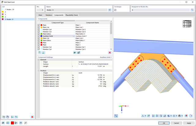
In the Steel Joints add-on, you can perform precise cuts on plates and structural components using the "Auxiliary Solid" component. Within this component, you can use the shapes of a box, a cylinder, or any cross-section as a guide object.
Go to Explanatory Video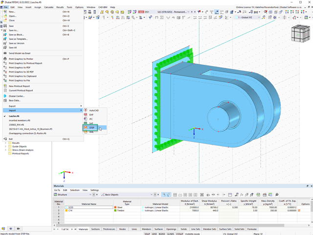
You can import STEP files into RFEM 6. The data is directly converted into the native RFEM model data.
The STEP format represents a standard interface initiated by ISO (ISO 10303). In the geometry description, all shapes relevant for RFEM (line, surface, and solid models) can be integrated by the CAD data models.
Note: This format is not to be confused with DSTV interfaces, which also use the file extension *.stp.
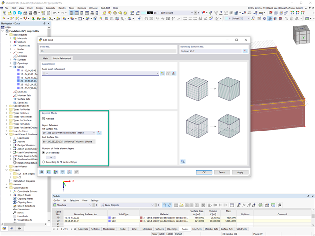
For the meshing of solids, you have the option of arranging a layered FE mesh. This option allows you to perform a defined division of the solid with finite elements between two parallel surfaces.
Go to Explanatory Video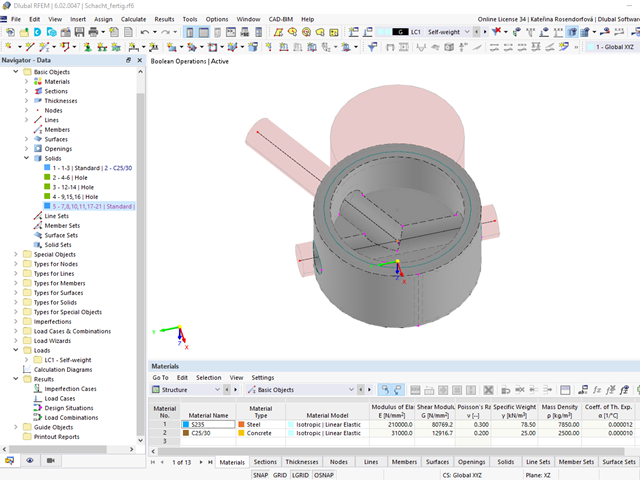
Curved elements are available only in RFEM. It's possible to intersect curved surfaces and solids.
When doing this, the program generates surfaces with the "Trimmed" surface type. With this technology, you can create very complex geometries, such as pipe intersections or curved openings, with a single click.
The intersection of solids is carried out adaptively using the new solid types "Hole" and "Intersection", according to the set theory. Use this method to create new, complex solid geometries similar to the manufacturing process (drilling, milling, turning, etc.). Therefore, it is possible to create complex curved surface or perforated solid elements. It's a simple process!
Go to Explanatory Video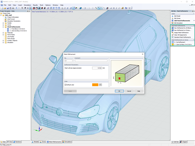
Do you already know the editor for mesh refinement control? It is a great help for your work! Why? It's easy – it gives you the following options:
- Graphic visualization of the areas with mesh refinements
- Mesh refinement of zones
- Deactivating the standard 3D solid mesh refinement with transversion into the corresponding manual 3D mesh refinements.
These options help you to formulate a suitable rule for meshing the entire model, even for the models with unusual dimensions. Use the editor to efficiently define small model details on large buildings or detailed meshing areas in the coating area of the model. You will be amazed!
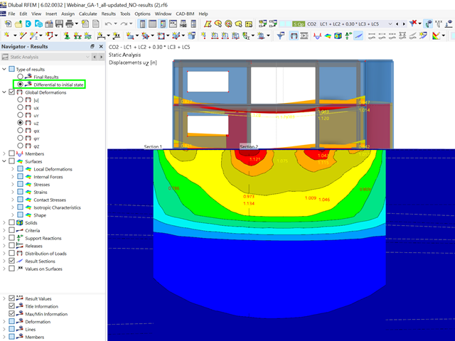
Did you already know? For load combinations, you can optionally display the difference results to the initial state. For example, you have the option for a geotechnical analysis to output the settlement as a difference to the initial state "soil self-weight".
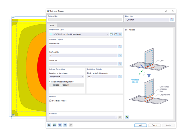
You probably already know that node, line, and surface releases are used to define transfer conditions between objects. For example, you can release members, surfaces, and solids from a line. It is also easily possible for the releases to have nonlinear properties, such as "Fixed if positive n", "Fixed if negative n", and so on.
.png?mw=640&hash=55038d2a1591f62179796666cb9b2fede0274e19)
A graphical and tabular output of the results for deformations, stresses, and strains helps you when determining the soil solids. To achieve this, use the special filter criteria for targeted selection of results.
The program doesn't leave you alone with the results. If you want to graphically evaluate the results in the soil solids, you can use the guide objects. For example, you can define clipping planes. This allows you to view the corresponding results in any plane of the soil solid.
And not just that. The utilization of result sections and clipping boxes facilitates the precise graphical analysis of the soil solid.
You already know that it is possible to model and analyze a soil and a structure in the entire model. As a result, you have explicitly taken into account the soil-structure interaction. By modifying a component, you achieve the immediate correct consideration in the analysis as well as in the results for the entire system of the soil and structure.

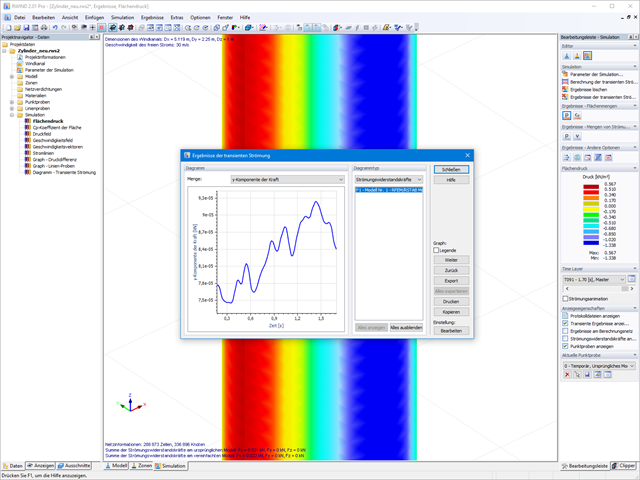
Are you ready for the evaluation? Use the calculation diagrams, which show the distribution of a specific result during the calculation.
You can freely define the layout of the vertical and horizontal axes of the calculation diagram. This allows you, for example, to consider the settlement distribution of a certain node, depending on the load.

Your data are always documented in a multilingual printout report. You can adjust the content at any time and save it as a template. You can also add graphics, texts, MathML formulas, and PDF documents to your report with just a few clicks.

Enter and model a soil solid directly in RFEM. You can combine the soil material models with all common RFEM add-ons.
This allows you to easily analyze the entire models with a complete representation of the soil-structure interaction.
All parameters required for the calculation are automatically determined from the material data that you have entered. The program then generates the stress-strain curves for each FE element.

Did you know? You can enter the soil layers that you have obtained from the subsoil expertises done in the locations into the program in the form of soil samples. Assign the explored soil materials, including their material properties, to the layers.
For the definition of the samples, you can enter the data in tables as well as in the respective editing dialog box. Furthermore, you can also specify the groundwater level in the soil samples.

The soil solids that you want to analyze are summarized in soil massifs.
Use the soil samples as a basis for a definition of the respective soil massif. This way, the program allows for user-friendly generation of the massif, including the automatic determination of the layer interfaces from the sample data, as well as the groundwater level and the boundary surface supports.
Soil massifs provide you with the option to specify a target FE mesh size independently of the global setting for the rest of the structure. You can thus consider the various requirements of the building and soil in the entire model.

Do you want to model and analyze the behavior of a soil solid? To ensure this, special suitable material models have been implemented in RFEM.
You can use the modified Mohr-Coulomb model with a linear-elastic ideal-plastic model or a nonlinear elastic model with an oedometric stress-strain relation. The limit criterion, which describes the transition from the elastic area to that of the plastic flow, is defined according to Mohr-Coulomb.
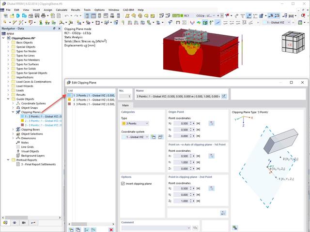
This feature also contributes to the clearly-arranged display of your results. Clipping planes are intersecting planes that you can place freely throughout the model. The zone in front of or behind the plane is consequently hidden in the display. This way, you can clearly and simply show the results in an intersection or a solid, for example.
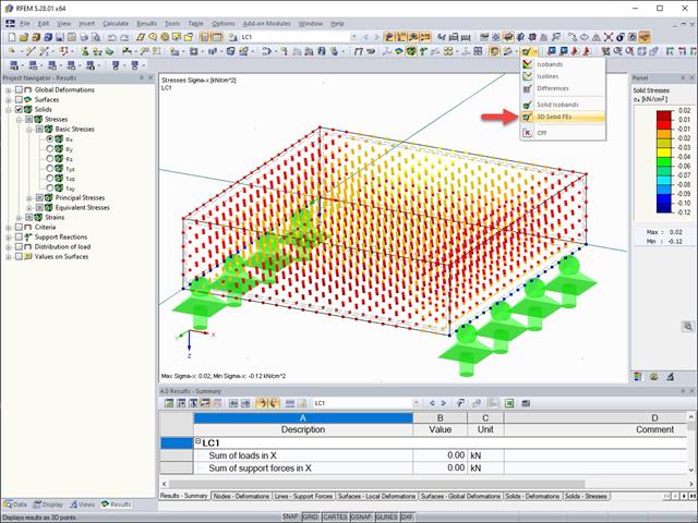
The results of solid stresses can be displayed as colored 3D points in the finite elements.
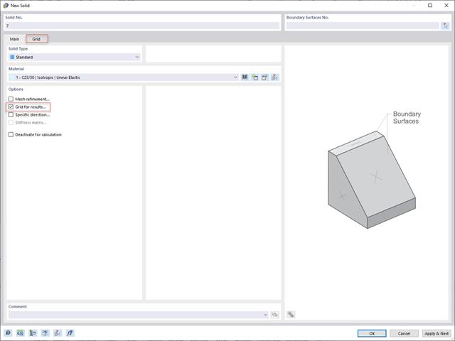
In addition to the "Mesh Refinement" and "Specific Direction" options for solids, you can also activate the "Grid for Results" option, which allows for organizing grid points in the solid space. Among other things, the center of gravity can be set as the origin. There is also the option to activate or deactivate the visibility of the grid for numerical results in "Navigator – Display" under Basic Objects.
.png?mw=640&hash=342149908caead326e60e26a2b5d05f7f46825cb)
Are you familiar with the Tsai-Wu material model? It combines plastic and orthotropic properties, which allows for special modeling of materials with anisotropic characteristics, such as fiber-reinforced plastics or timber.
If the material is plastified, the stresses remain constant. The redistribution is carried out according to the stiffnesses available in the individual directions. The elastic area corresponds to the Orthotropic | Linear Elastic (Solids) material model. For the plastic area, the yielding according to Tsai-Wu applies:
All strengths are defined positively. You can imagine the stress criterion as an elliptical surface within a six-dimensional space of stresses. If one of the three stress components is applied as a constant value, the surface can be projected onto a three-dimensional stress space.
If the value for fy(σ), according to the Tsai-Wu equation, plane stress condition, is smaller than 1, the stresses are in the elastic zone. The plastic area is reached as soon as fy (σ) = 1; values greater than 1 are not allowed. The model behavior is ideal-plastic, which means there is no stiffening.

Did you know? In contrast to other material models, the stress-strain diagram for this material model is not antimetric to the origin. You can use this material model to simulate the behavior of steel fiber-reinforced concrete, for example. Find detailed information about modeling steel fiber-reinforced concrete in the technical article about Determining the material properties of steel-fiber-reinforced concrete.
In this material model, the isotropic stiffness is reduced with a scalar damage parameter. This damage parameter is determined from the stress curve defined in the Diagram. The direction of the principal stresses is not taken into account. Rather, the damage occurs in the direction of the equivalent strain, which also covers the third direction perpendicular to the plane. The tension and compression area of the stress tensor is treated separately. In this case, different damage parameters apply.
The "Reference element size" controls how the strain in the crack area is scaled to the length of the element. With the default value zero, no scaling is performed. Thus, the material behavior of the steel fiber concrete is modeled realistically.
Find more information about the theoretical background of the "Isotropic Damage" material model in the technical article describing the Nonlinear Material Model Damage.
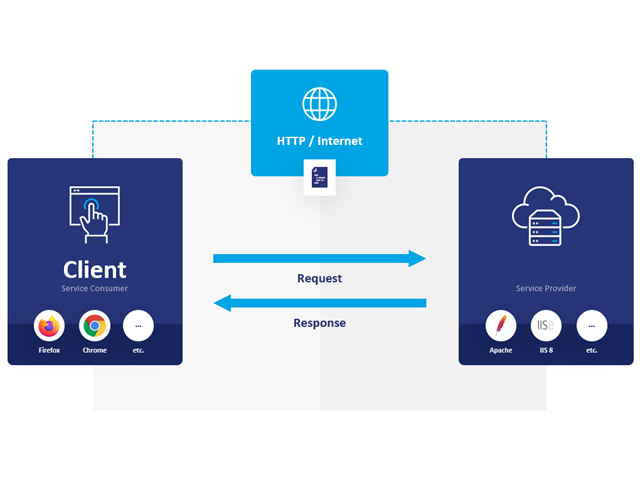
WebService and API provide you various scope of application. We have summarized some ideas as to how WebService and API can support your company:
- Creating additional applications for RFEM 6, RSTAB 9, and RSECTION 1
- Possibility to make the workflows more efficient (for example, model definition and input) and to integrate RFEM 6, RSTAB 9, and RSECTION 1 into your company applications
- Simulating and calculating several design options
- Running optimization algorithms for size, shape, and/or topology
- Accessing the calculation results
- Generation of printout reports in the PDF format
The level of quality of the work is automatically increased not only by the algorithmic model definitions, but also by:
- Extending / consolidating RFEM 6, RSTAB 9, and RSECTION 1 with your own controls
- Increased interoperability between the individual software used to complete a project
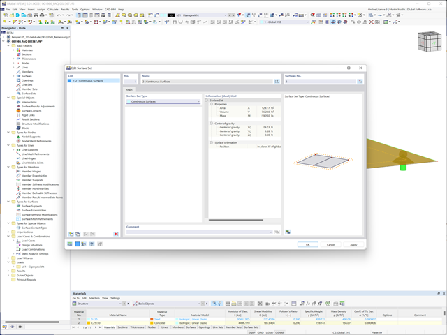
The aim of this feature is to make your design more efficient. In addition to member sets, you can also combine lines, surfaces, and solids into sets. For example, you can consider them as uniform elements in the design.
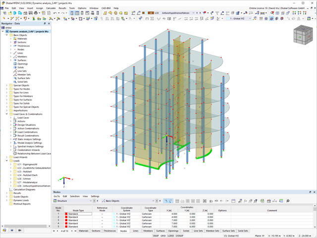
RFEM is entering a new phase with RFEM 6! The new generation of the 3D FEA software is also used for the structural analysis of members, surfaces, and solids. Many of the tried and tested features remain, but we have improved them and added new features to make your work with RFEM even easier.
What particularly distinguishes RFEM 6 is the modern design concept, with the add-ons integrated directly into the program. Curious to learn more?
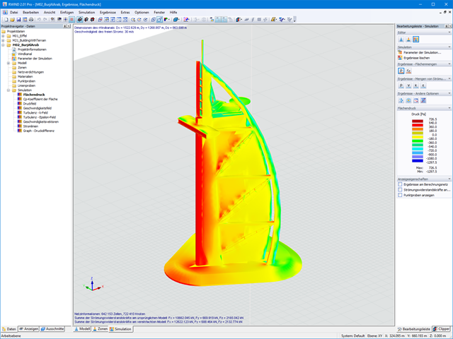
By solving the numerical flow problem, you can obtain the following results on and around the model:
- Pressure on structure surface
- Coefficient Cp distribution on the structure surfaces
- Pressure field about the structure geometry
- Velocity field about the structure geometry
- Turbulence k-ω field about the structure geometry
- Turbulence k-ε field about the structure geometry
- Velocity vectors about the structure geometry
- Streamlines about the structure geometry
- Forces on member-shaped structures that were originally generated from member elements
- Convergence diagram
- Direction and size of the flow resistance of the defined structures
Despite this amount of information, RWIND 2 remains clearly arranged, as is typical for the Dlubal programs. You can specify freely definable zones for a graphic evaluation. Voluminously displayed flow results about the structure geometry are often confusing – you know the problem for sure. That's why RWIND Basic provides freely movable section planes for the separate display of the "solid results" in a plane. For the 3D branched streamline result, you have an option to select between a static and an animated display in the form of moving line segments or particles. This option helps you to represent the wind flow as a dynamic effect.
You can export all results as a picture or, especially for the animated results, as a video.
When starting the analysis in the RFEM or RSTAB application, you trigger a batch process. It places all member, surface, and solid definitions of the model rotated with all relevant coefficients in the numerical wind tunnel of RWIND Basic. Furthermore, it starts the CFD analysis, and returns the resulting surface pressures for a selected time step as FE mesh nodal loads or member loads into the respective load cases of RFEM or RSTAB.
These load cases which contain RWIND Basic loads can then be calculated. Moreover, you can combine them with other loads in load and result combinations.
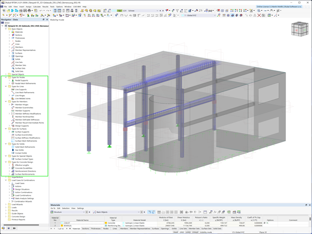
Use the specification of the element types for members, surfaces, solids, and so on, to facilitate your input (such as member nonlinearities, member stiffnesses, design supports, and many others).
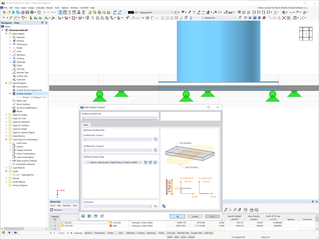
Make your work easier. A surface contact serves to describe a contact definition between two or more surfaces that are at a distance from each other It is no longer necessary to create a contact solid between the surfaces.
Go to Explanatory Video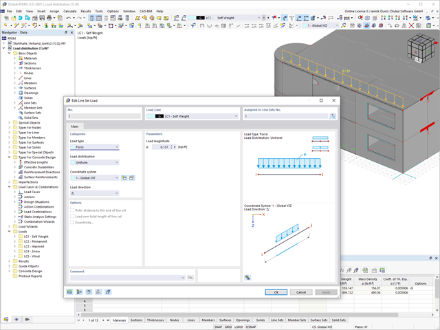
Now, you have new options for your design: With the introduction of line sets, surface sets, and solid sets, new load options have also been added for loading these sets. Try them yourself!

Compared to the RF‑SOILIN add-on module (RFEM‑5), the following new features have been added to the Geotechnical Analysis add-on for RFEM 6:
- Creation of the layered soil as a 3D model from the entirety of the defined soil samples
- Recognized material law according to Mohr-Coulomb for soil simulation
- Graphical and tabular output of stresses and strains at any depth of the soil
- Optimal consideration of the soil-structure interaction on the basis of an overall model

Compared to the RF‑/STEEL add-on module (RFEM 5 / RSTAB 8), the following new features have been added to the Stress-Strain Analysis add-on for RFEM 6 / RSTAB 9:
- Treatment of members, surfaces, solids, welds (line welded joints between two and three surfaces with subsequent stress design)
- Output of stresses, stress ratios, stress ranges, and strains
- Limit stress depending on the assigned material or a user-defined input
- Individual specification of the results to be calculated through freely assignable setting types
- Non-modal result details with prepared formula display and additional result display on the cross-section level of members
- Output of the design check formulas used